Bregman Divergences July 16, 2018

Bregman divergences pop up everywhere in machine learning literature. It's important to understand what they are, where they come from, and why they are so useful in many areas of machine learning. In this previous post on convexity we covered convex sets and convex functions, and briefly touched on Bregman divergences. This post will go in to a lot more detail about Bregman divergences: we'll derive several from scratch, and we'll look at their useful properties and the roles they play in machine learning. I've also flexed my javascript muscles and created some interactive graphs to play with :)

The Taylor Approximation of a Vector-Valued Function

Before we get stuck in to Bregman divergences, let's do a quick review the Taylor series approximation of functions with vector inputs.
Most readers should be familiar with the Taylor series approximation in \(1\)-dimension: the approximation of a function \(f(x)\) around a point \(x_{0}\) is given by:

\[f\left( x\right) = f\left( x_{0}\right) + f'\left( x_{0}\right)\left(x - x_{0}\right) + \frac{f''\left( x_{0}\right)}{2!}\left( x - x_{0}\right)^{2}+ \frac{f'''\left( x_{0}\right)}{3!}\left( x - x_{0}\right)^{3} + ... \]

but remember this is only for a function \(f : \mathbb{R} \rightarrow \mathbb{R}\). For functions that take in vector arguments, i.e. \(g :\mathbb{R}^{n} \rightarrow \mathbb{R}\), we will need the appropriate Taylor expansion:

\[g\left(\mathbf{x}\right) = g\left(\mathbf{x}_{0}\right) + \mathbf{\nabla} g\left(\mathbf{x}_{0}\right)^{T}\left(\mathbf{x} - \mathbf{x}_{0}\right) + \left(\mathbf{x} -\mathbf{x}_{0}\right)^{T} H\left(\mathbf{x}\right)\left(\mathbf{x} -\mathbf{x}_{0}\right)+ ... \]

where \(H(\mathbf{x})\) is the Hessian of \(g\), i.e. a matrix of second derivatives where \(H_{ij} = \frac{\partial}{\partial x_{j}}\frac{\partial g}{\partial{x_{i}}}\).


For Bregman divergences, we'll only need the \(1\)st-order Taylor (or linear) approximation, \(g(\mathbf{x}) \approx g(\mathbf{x}_{0}) + \mathbf{\nabla} g(\mathbf{x}_{0})^{T}(\mathbf{x} - \mathbf{x}_{0})\).

If our function is \(1\)-dimensional, this linear approximation would act like a tangent to the function at \(\mathbf{x_{0}}\). If our function was \(2\)-dimensional and convex (which would look like a bowl), the linear approximation would then be a plane touching the bowl at \(\mathbf{x_{0}}\).

Bregman Divergences

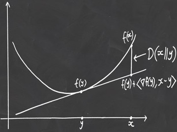
So let's get to it! The elusive Bregman divergences. Bregman divergences are a fantastic tool in developing and analysing many machine learning algorithms. In essence, they are a type of distance function, in that they measure the distance between two points in a very particular way. We would write the Bregman divergence between \(\mathbf{x}\) and \(\mathbf{y}\) as \(D\left(\mathbf{x}\|\mathbf{y}\right)\). But they are not a true distance metric. Before we get into that though, let's see where they come from:


All Bregman divergences come from convex functions. We say they are induced by a convex function. That's because if we start with some function \(f : \mathbb{R}^{n} \rightarrow \mathbb{R}\) (which is convex) then we can define the bregman divergence \(D(\mathbf{x}\|\mathbf{y})\) as:

\[D\left(\mathbf{x}\|\mathbf{y}\right) = f\left(\mathbf{x}\right) - \left[f\left(\mathbf{y}\right) + \langle\mathbf{\nabla} f\left(\mathbf{y}\right), \left(\mathbf{x} - \mathbf{y}\right)\rangle\right]\]

which if you look closely, is simply the difference between the function and the \(1\)st-order approximation of the function at \(\mathbf{y}\), when evaluated at \(\mathbf{x}\), as seen below.







So now we know how to create a Bregman divergence, let's try it out! If we take the function \(f\left(\mathbf{x}\right) = \|\mathbf{x}\|^{2}\) (the Euclidean norm squared), which is a convex function, then the Bregman divergence would be

\[\begin{align}D\left(\mathbf{x}\|\mathbf{y}\right) &= \|\mathbf{x}\|^{2} - \|\mathbf{y}\|^{2} -\langle\mathbf{\nabla} f\left(\mathbf{y}\right), \left(\mathbf{x} - \mathbf{y}\right)\rangle\\
&= \|\mathbf{x}\|^{2} - \|\mathbf{y}\|^{2} - \langle 2\mathbf{y} , \left(\mathbf{x} - \mathbf{y}\right)\rangle\\
&= \|\mathbf{x}\|^{2} - \|\mathbf{y}\|^{2} - 2\langle\mathbf{y} , \mathbf{x}\rangle + 2\|\mathbf{y}\|^{2}\\
&= \|\mathbf{x}\|^{2} + \|\mathbf{y}\|^{2} - 2\langle\mathbf{y} , \mathbf{x}\rangle\\
&= \|\mathbf{x} - \mathbf{y}\|^{2}\end{align}\]

which you can see below, and play with! Click and drag the points \(f(x)\) and \(f(y)\) around on the blue curve \((f(\mathbf{x}) = \|\mathbf{x}\|^{2})\) to move them. The red line is the Bregman divergence.

Another convex function that induces a very useful Bregman divergence is the negative entropy, \(f(\mathbf{x}) = \sum_{i=1}^{n} x_{i}\log x_{i}\), where the points \(\mathbf{x}\) are confined to the probability simplex \(\Delta_{x}\), which is simple the convex set defined as \(\Delta_{x} = {\mathbf{x} : x_{i} \geq 0, \sum_{i}^{n} x_{i} = 1}\)

The Bregman divergence induced by the negative entropy is then:

\[\begin{align}D\left(\mathbf{x}\|\mathbf{y}\right) &= \sum_{i=1}^{n} x_{i}\log x_{i} - \sum_{i=1}^{n} y_{i}\log y_{i} -\langle\mathbf{\nabla} f\left(\mathbf{y}\right), \left(\mathbf{x} - \mathbf{y}\right)\rangle\\
&= \sum_{i=1}^{n} x_{i}\log x_{i} - \sum_{i=1}^{n} y_{i}\log y_{i} -\langle\mathbf{1} + \log \mathbf{y}, \left(\mathbf{x} - \mathbf{y}\right)\rangle\\
&= \sum_{i=1}^{n} x_{i}\log x_{i} - \sum_{i=1}^{n} y_{i}\log y_{i} -\sum_{i=1}^{n} x_{i}\log y_{i} + \sum_{i=1}^{n} y_{i}\log y_{i} - \sum_{i=1}^{n} x_{i} + \sum_{i=1}^{n} y_{i}\\
&= \sum_{i=1}^{n} x_{i}\log x_{i} - \sum_{i=1}^{n} x_{i}\log y_{i} - 1 + 1\\
&=\sum_{i=1}^{n} x_{i}\log \frac{x_{i}}{y_{i}}\end{align}\]

where \(\log \mathbf{y}\) is the element-wise logarithm of the vector \(\mathbf{y}\). This Bregman divergence is very well known, and is called the Kullback-Leibler divergence or relative entropy. It's where this blog gets its name! Again you can play with this divergence below.

The Kullback-Liebler divergence is used in fields such as Information Theory, since \(D\left( P\| Q\right)\) is the divergence of \(P\) away from \(Q\).

From the above graphs, you can begin to see why Bregman divergences are used as a 'sort-of' distance function. Due to the convexity of our starting function, the 1st-order Taylor approximation (tangent or hyperplane) will always lie below the function. This means that \(D(\mathbf{x}\|\mathbf{y})\geq 0\) for all \(\mathbf{x}\) and \(\mathbf{y}\), and \(D(\mathbf{x}\|\mathbf{y}) = 0\) only when \(\mathbf{x} = \mathbf{y}\), just like any other distance function. If you recall however, at the beginning of this post we said that Bregman divergences are not true distance metrics, that's because they are not usually symmetric (\(D(\mathbf{x}\|\mathbf{y})\neq D(\mathbf{y}\|\mathbf{x})\)), and they don't follow the triangle inequality.

Useful Properties of Bregman Divergences in Machine Learning

The more reading you do in to machine learning theory, the more you will come across Bregman divergences, so here's a list of their useful properties:

1. Bregman Projections:
Since they are a (sort of) distance function, they can be used to project vectors onto convex sets. Many machine learning algorithms employ Bregman projections, defined as \(\mathbf{y}^{*} = \arg\min_{\mathbf{y}\in S} D(\mathbf{x}\|\mathbf{y})\), and from the convexity of the set \(C\), and the convexity of the Bregman divergence in its first argument, this solution exists and is unique.

2. Pythagorean Theorem:
For Bregman divergences, a generalised Pythagorean theorem exists: if \(C\) is a convex set in \(\mathbb{R}^{n}\), then for all \(\mathbf{x}\in C\), and \(\mathbf{y}\in\mathbb{R}^{n}\), if \(\mathbf{z}\) is the projection of \(\mathbf{y}\) onto \(C\) then: \[D(\mathbf{x}\|\mathbf{y}) \geq D(\mathbf{x}\|\mathbf{z}) + D(\mathbf{z}\|\mathbf{y})\]

3. Convexity in its first argument:
As a function, for a fixed \(\mathbf{x}\), \(D(\mathbf{x}\|\mathbf{y})\) is itself a convex function for all \(\mathbf{y}\).

4. Algorithms:
Bregman divergences appear very often in the construction and analysis of online machine learning algorithms. Some examples are Boosting as Entropy Projection, or the Multiplicative Weights Update method, but there are countless other examples out there as well.

References & Sources

• Kivinen, J. and Warmuth, M.K., 1999, July. Boosting as entropy projection. In Proceedings of the twelfth annual conference on Computational learning theory (pp. 134-144). ACM.
• Arora, S., Hazan, E. and Kale, S., 2012. The Multiplicative Weights Update Method: a Meta-Algorithm and Applications. Theory of Computing, 8(1), pp.121-164.
• Boyd, S. and Vandenberghe, L., 2004. Convex optimization. Cambridge university press.
• I was inspired by this excellent blog post on the Bregman divergences, which also includes interactive graphs, so credit for that idea goes to the author (Mark Reid), the code for my interactive graphs is my own however, and can be found here.