Spectral Clustering Feb. 22, 2018

Why is it Useful?

When faced with a clustering problem, the knee-jerk reaction is to go for a simple algorithm like K-means. There is a startling problem with such techniques however; K-means clustering -and its close relatives- are only effective on data which is compactly clustered, and separable by convex boundaries. What happens when our data is connected?

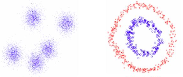
Fig 1. An example of data that's easy to cluster (left) and more difficult to cluster (right)

You can see from the above image that K-means would be successful in clustering the data on the left, but is going to have a tough time trying to cluster the data on the right. There is no convex boundary that can separate this data, so what do we do? Turn to spectral clustering of course!

Graphs

Any set of data can be represented as a graph (or network), where each data point is represented by a node (or vertex), and certain nodes are connected via an edge.

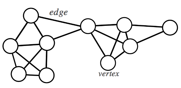
Fig 2. A simple example of a graph

A graph \(G = (V,E)\) with vertex set \(V = {v_{1},v_{2},...,v_{n}}\) can be either weighted or unweighted. If our graph is weighted, then we must choose a system to define the weights of the edges between pairs of vertices. The obvious choice here is that our weighted edges should represent some measure of similarity between two data points. When two data points are very similar to each other, they should have a very strongly weighted edge between them. When two data points are very dissimilar, then they should have a a very weak edge between them, or none at all. If we do this then we can then represent our graph with a weighted affinity (or adjacency) matrix \(W = (w_{ij})_{i,j=1,...,n}\).

One could use a very simple measure of similarity, such as Euclidean distance, but the most common method is to use a Gaussian kernel similarity function:

\[W_{ij} = \mathrm{e}^{\frac{-|| x_{i} - x_{j} ||^{2} }{2\sigma^{2}}}\]

which is particularly useful because we can control the width of the Gaussian curve with \(\sigma\), and we can even create a cut off point, \(C\) so that if \(W_{ij} < C\) we can set it to zero, thus disconnecting very dissimilar pairs of vertices in our network. Doing this has the added benefit of giving us a mostly sparse matrix \(W\) containing only the most important weights of our network. This sparsity is important, as we will see.

Clustering with Graphs?

So we have a dataset represented as a graph, isn't there a way to just cluster the data directly from the graph? Actually there is, in graph theory there are techniques to partition graphs into clusters, known as cutting.

The most simple partitioning method is the min-cut, which seeks to find a set of clusters with minimised weights between each cluster.

\[Cut(A,B) := \sum_{i \in A, j \in B}^{} W_{ij}\]

Where \(A\) and \(B\) are clusters of vertices. Unfortunately this method does not give us very useful solutions. It will often return very small clusters (possibly consisting of a single node) because they are connected to the graph via a very small weight.

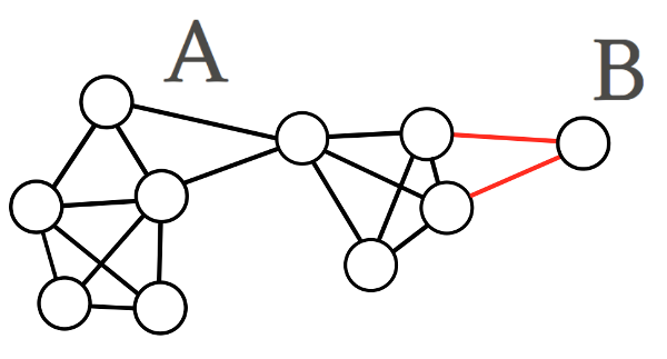
Fig 3. An example of a min-cut solution

Often we are looking for a more balanced solution, where our clusters are of similar volume, so we could consider the volume of the cluster we are making when cutting the graph. This is a method called the normalised min-cut.

To find the volume of a cluster we must first define the degree of a vertex:

\[d_{i} = \sum_{j=1}^n w_{ij}\]

which is just the sum of all weights connected to that vertex. We can then define the volume of a cluster \(A\) to be the sum of the degrees of each vertex in that cluster,

\[Vol(A) = \sum_{i \in A}^{} d_{i}\]

allowing us to define the normalised cut to be

\[Ncut(A,B) := \frac{cut(A,B)}{\left(\frac{1}{vol(A)} + \frac{1}{vol(B)}\right)}\]

whose minimised solution might return something like the following

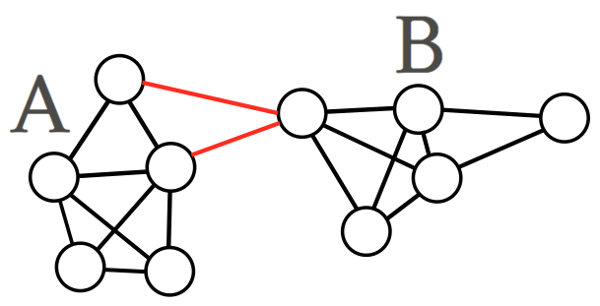
Fig 4. An example of a normalised min-cut solution

This normalised min-cut gives much better solutions, but this method is only solvable if one considers every possible cut and compares it to all other possible variations, and is therefore NP-hard. Spectral clustering performs a relaxation of this normalised-cut NP-hard problem.

Spectral Clustering and the Laplacian

The word 'spectral' in spectral clustering is referring to the eigenvalues of a special matrix used to describe our graph. In linear algebra the set of eigenvalues of a matrix is referred to as its spectrum. This special matrix is called the Graph Laplacian, which has some interesting and very useful properties.

So far the only matrix we have to describe our graph is the Affinity matrix, \(W\). To get our graph Laplacian, we must construct another matrix called the Degree matrix, which is a diagonal matrix whose diagonal elements simply contain the degree of that vertex in our graph:

\[D_{i i} = \sum_{j}^{n} d_{i,j}\]

In the literature many different Laplacians are used, we will look at some of them here, but refer to Chung (1997) for a more in-depth look. The most simple Laplacian is the unnormalised Laplacian, which is simply the difference between our Degree matrix and our Affinity matrix:

\[L = D - W\]

Another common Laplacian used is the normalised Laplacian, given by

\[L_{n} = D^{-\frac{1}{2}}WD^{\frac{1}{2}}\]

or sometimes

\[L_{rw} = D^{-1}L = I - D^{-1}W\]

where 'rw' is in reference to the fact that this Laplacian is very closely related to a random walk across a graph.

Eigen-solutions to the normalised Laplacian can be found by using the unnormalised Laplacian and solving the eigenvalue problem for \(Lv = \lambda Dv\) (which is really just finding the eigen-solutions for \(L_{rw}\) - see above). By doing this, we obtain the spectrum of the graph Laplacian and the corresponding set of eigenvectors.

If our graph is disconnected (so that our Affinity matrix is sparse), then our Laplacian is approximately block-diagonal. Each block in the Laplacian represents the Laplacian for each connected component in the graph. In the case where we have 3 connected components, the Laplacian (and its first 3 eigenvectors) would look like the following:

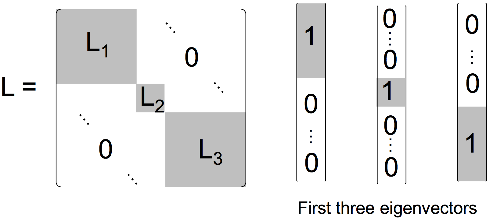
Fig 5. A block-diagonal Laplacian matrix with corresponding eigenvectors

If our graph is connected, then these off-diagonal 'zero-blocks' will have some small non-zero perturbations in them. In this situation our Laplacian's first eigenvector is constant (consisting purely of 1's), and the second and third eigenvectors represent the normalised min-cut. For a concrete example see the example below.

You might be wondering why we have to choose the first k-eigenvectors? Well, as is the case with all clustering algorithms, we must choose the number of clusters for our algorithm to find. For spectral clustering this corresponds to selecting the \(k\) lowest eigenvalues (and their corresponding eigenvectors) for each block in the Graph Laplacian.

Before we look at an example, let's explore some more properties of the Laplacian matrix.

1. \(L\) is a singular, symmetric, positive-semidefinite matrix (its eigenvalues are all greater than or equal to zero).

2. The row sum and column sum of \(L\) is always zero.

3. The smallest eigenvalue of \(L\), \(\left(\lambda_{0}\right)\), is zero.

4. The smallest non-zero eigenvalue of \(L\) is known as the spectral gap.

5. The number of connected components of a graph is represented by the number of eigenvalues of the Laplacian that are equal to zero.

This last property sheds some light on the difference between the eigen-solutions to the disconnected graphs and the connected graphs we discussed earlier:

Recall that for the disconnected graph with \(k\)-connected components, the Laplacian can be split into \(k\) blocks along the diagonal, each corresponding to an independent Laplacian for those connected components. These Laplacians will each have their smallest eigenvalue be equal to zero. So for a disconnected graph with \(k\)-connected components, you can expect \(k\) 0-valued eigenvalues (here \(k\) is sometimes called the multiplicity of the eigenvalue 0).

For the connected graph, you could consider the whole graph as one cluster (because it is one connected component!) and so, the Laplacian will only have one eigenvalue equal to zero. The second smallest eigenvalue (and corresponding eigenvector) will contain the information about the two most 'strongly'-connected components within that graph, and so on.

A Toy Example

Let's take a look at a simple example with the unnormalised graph Laplacian (but remember we will be getting the eigen-solutions for the normalised Laplacian given by \(Lv = \lambda Dv\)). We will use 6 data points that we want to be able to split into \(k=2\) clusters. The data points are shown as a disconnected graph below.

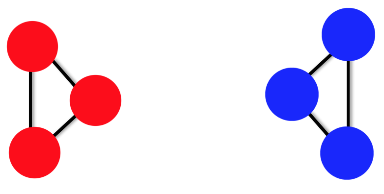
Fig 6. A toy example of a simple disconnected graph. All weights are equal to 1

We can construct a \(6\times6\) matrix for \(W\) and a\(6\times6\) diagonal matrix for D and use these to construct the unnormalised Laplacian. Finding the first two eigenvectors \(\left( F_{1} \mbox{and } F_{2}\right)\):

\[ L = D - W = \begin{array}{c} \begin{bmatrix} 2 & -1 & -1 & 0 & 0 & 0 \\ -1 & 2 & -1 & 0 & 0 & 0 \\ -1 & -1 & 2 & 0 & 0 & 0 \\ 0 & 0 & 0 & 2 & -1 & -1 \\ 0 & 0 & 0 & -1 & 2 & -1 \\ 0 & 0 & 0 & -1 & -1 & 2 \end{bmatrix} \\ \end{array} \longrightarrow \begin{array}{c} \left[ \begin{array}{c} 0.58 \\ 0.58 \\ 0.58 \\ 0 \\ 0 \\ 0 \end{array} \right] \\ F_{1} \end{array} \& \begin{array}{c} \left[ \begin{array}{c} 0 \\ 0 \\ 0 \\ 0.58 \\ 0.58 \\ 0.58 \end{array} \right] \\ F_{2} \end{array}\]

For simplicity I neglected to use the Gaussian kernel similarity function, but instead have set the Affinity matrix to be equal to the Adjacency matrix, that is,
\[W_{i,j} = \begin{cases} 1 & \mbox{if \(i\) & \(j\) are connected} \\ 0 & \mbox{otherwise, or if } i=j \end{cases}\]

Taking these first two eigenvectors \(\left( F_{1} \mbox{and } F_{2}\right)\) and treating them as an orthonormal basis, we can then project our data into this lower-dimensional space. This is achieved by putting these eigenvectors together column-wise, giving us an \(n \times k\) matrix and taking each row of this matrix as co-ordinates of each data point in the new \(\mathbb{R}^{k}\) space.

\[\begin{array}{c} \left[ \begin{array}{c} 0.58 \\ 0.58 \\ 0.58 \\ 0 \\ 0 \\ 0 \end{array} \right] \\ F_{1} \end{array} \& \begin{array}{c} \left[ \begin{array}{c} 0 \\ 0 \\ 0 \\ 0.58 \\ 0.58 \\ 0.58 \end{array} \right] \\ F_{2} \end{array} \longrightarrow \left[ \begin{array}{cc} 0.58 & 0 \\ 0.58 & 0 \\ 0.58 & 0 \\ 0 & 0.58 \\ 0 & 0.58 \\ 0 & 0.58 \end{array}\right]\]

which you can see plotted below

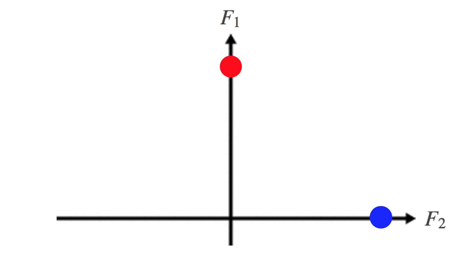
Fig 7. A plot of the data in the new lower-dimensional subspace spanned by the first two eigenvectors of the Laplacian. Note that F1 lies along the vertical axis, and F2 along the horizontal axis.

The effect of doing this is that by embedding our data points in \( \mathbb{R}^k\), they can now very easily be separated by convex boundaries, using a classic algorithm such as K-means. Great! In fact the data points corresponding to each cluster are lying on the same point in \( \mathbb{R}^k\), which isn't surprising given the symmetry of the disconnected graph we used.

Let's take this example further, and consider what happens when our graph is loosely connected.

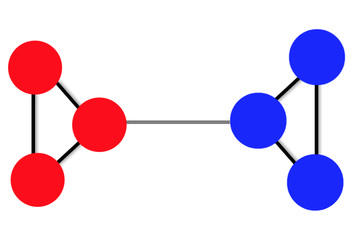
Fig 8. A toy example of a loosely-connected graph. The dark weights are equal to 1 (just as in the fig 5.). The light-grey weight is equal to 0.2.

The effect of this is to add some small perturbation to our Affinity matrix. If we construct the Graph Laplacian again,
\[ L = D - W = \begin{array}{c} \begin{bmatrix} 2 & -1 & -1 & 0 & 0 & 0 \\ -1 & 2 & -1 & 0 & 0 & 0 \\ -1 & -1 & 2.2 & -0.2 & 0 & 0 \\ 0 & 0 & -0.2 & 2.2 & -1 & -1 \\ 0 & 0 & 0 & -1 & 2 & -1 \\ 0 & 0 & 0 & -1 & -1 & 2 \end{bmatrix} \\ \end{array} \]
and find the first \(k=2\) eigenvectors:
\[\begin{array}{c} \left[ \begin{array}{c} 0.41 \\ 0.41 \\ 0.41 \\ 0.41 \\ 0.41 \\ 0.41 \end{array} \right] \\ F_{1} \end{array} \& \begin{array}{c} \left[ \begin{array}{c} 0.42 \\ 0.42 \\ 0.37 \\ -0.37 \\ -0.42 \\ -0.42 \end{array} \right] \\ F_{2} \end{array} \longrightarrow \left[ \begin{array}{cc} 0.41 & 0.42 \\ 0.41 & 0.42 \\ 0.41 & 0.37 \\ 0.41 & -0.37 \\ 0.41 & -0.42 \\ 0.41 & -0.42 \end{array}\right]\]

We can see that the block-behaviour of the elements of the eigenvectors in the previous example is still reflected here by the change of sign in \(F2\). This is shown more clearly if we embed the data in \(\mathbb{R}^k\) again:

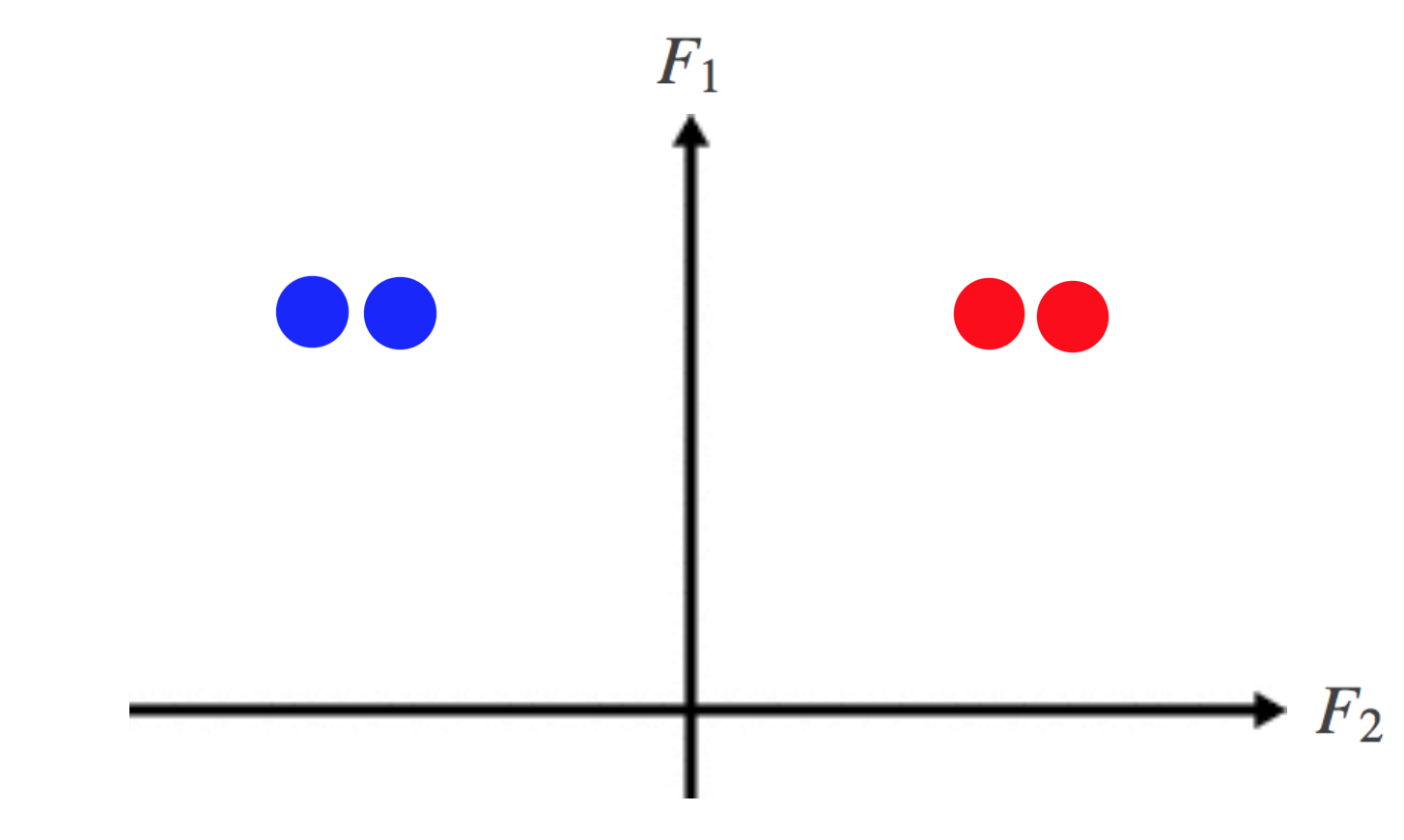
Fig 9. A plot of the loosely-connected data in the lower-dimensional subspace spanned by the first two eigenvectors of the Laplacian. Again, note that F1 lies along the vertical axis, and F2 along the horizontal axis.

and again, just like before, the data is now separable by a simple clustering algorithm such as K-means. The reason spectral clustering works even under small perturbations to the Affinity matrix is because the \(subspace\) spanned by the eigenvectors of \(L\) are stable to these small changes.

Sources

The resources I used most while learning this topic were:

Spectral Graph Theory (Chung 1997)

A Tutorial on Spectral Clustering (Luxburg 2007)

Spectral Clustering (Lecture Slides) (Singh - Carnegie Mellon - 2010)